
If you haven't seen the map, go and check it out: lab.jcode.me/openWiFiMap/
Introduction
Like most of my projects this one started with a question: how much of my city was covered by open Wi-Fi signals and how strong those signals are.
What I wanted to create was something close to a phone signal coverage map but for open Wi-Fi.
I would need to:
- Gather data
- Filter that data
- Visualise the data using some form of map
- Make it interactive
The first step
To answer my own question I needed to gather data, hopefully without lugging around a laptop or other heavy hardware.
I've done wardriving in the past, using a laptop running Linux and a wireless USB adapter, however this seemed overkill and would likely start to draw too much attention.
After some quick testing I chose to gather my data using a spare Android phone I keep around for tinkering. I designed the Android app to be very minimal in both the user interface and the code behind it.
The app
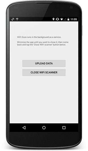
On the surface the app has two buttons; "Close WiFi scanner" and "Upload data". Behind the scenes it's only a little cooler. Upon opening the app it starts a background service that hooks into the phones location services - this covers GPS and network location methods - and listens for updates or movements. After testing different movement configurations I decided to use a minimum of 10 meters or 5 seconds since the last update.
Upon 'hearing' a change in location the background service then triggers a Wi-Fi scan, which returns the most important part, names and signal strength. It then stores the following data for later filtering;
- BSSID - Access point MAC address, used for unique identification purposes
- SSID - Access point name
- RSSI - Access point signal strength
- Security - Access point encryption methods, for filtering open connections
This all runs in the background until the "Upload data" button is pressed. Once pressed it compresses the collected information and uploads it to one of my servers which checks the integrity of the information then stores and filters the raw information into a SpatiaLite database ready for QGIS to interpret.
NB: I didn't start with QGIS, my first test used Google Maps and heatmap.js to create an overlay of the signal strength map, but I quickly ran into issues like disappearing points, heatmap scaling errors and slow maps with far too many points.
Quantum Geographic Information System (QGIS)
Geographic Information Systems or GIS is something I've never used before, so this is where I had most of my fun, where I started yelling incoherently, where I did most of my learning and finally got the result I wanted from the start.
Luckily for me QGIS can read SpatiaLite files, so importing the first round of data was as simple as opening the file and selecting the correct CRS (WGS 84 for this project, GDA94 did not play nice with other layers) and watching the points fill up the screen.
By this time I had given the Android app to some awesome friends who helped me gather data, and I was amassing enough to start the visualisation process.
The first import was quite impressive but single colour data points look so boring, so I threw on a graduated colour style using signal strength as the index.


With data being accurately plotted my next goal was create a hexbin map.
Creating a hexbin map inside QGIS requires only 1 plugin; MMQGIS.
MMQGIS allows you to create a grid polygon layer of any size over a selected area, the larger the area and the smaller the hexagons the longer it takes to generate a polygon layer.
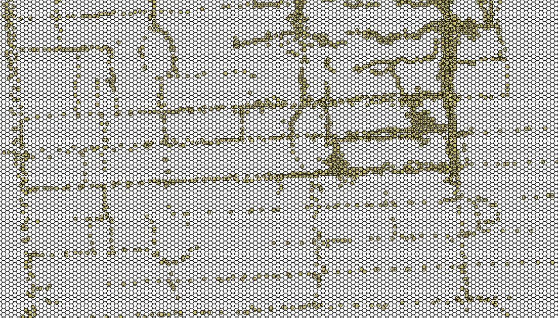
After the hexagonal layer was drawn I used a "Points in Polygon" method and had success, but the amount of points in a polygon isn't indicative of Wi-Fi signal strength.

One suggested solution was to use "Zonal Statistics". This did not work out the way it should have...the blasted map it made was upside-down!

Just before I was going to give up on hexbins and settle for a generic heatmap I stumbled upon "Join attributes by location".
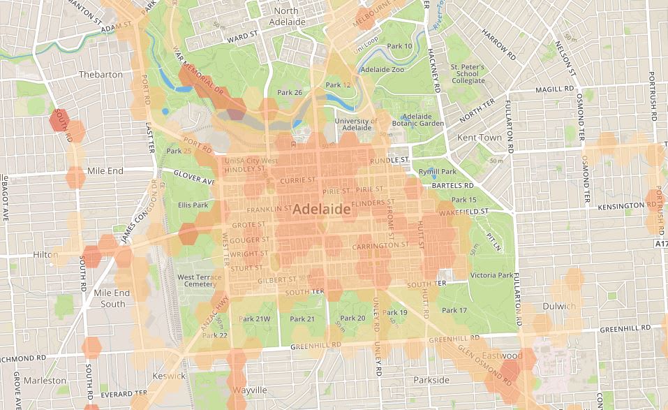
This looked promising. Using the point layer with the polygon vector layer I took a mean and median summary of intersecting attributes, discarding all empty polygons and stored it in a new layer.
Applying the same graduated colour style as before created the map I wanted. I was almost done.
Creating tiles
QGIS maps are not particularly portable, in order to read .shp layers dedicated programs must be installed. These programs are hundreds of megabytes in size, and while it's not a worry for some, downloading large applications just to view a map isn't worth it. So I sought other methods of sharing my map.
Leaflet, a modern open-source JavaScript library for mobile-friendly interactive maps would allow me to create my interactive map using custom tile layers.
There are many methods of creating tile layers; QGIS Server, TileCache and MAPNIK allow users to create and server their own maps, Mapbox even handles .shp files and makes a whole map ready to show off with very little effort, but I wanted to do it and host it myself.
Using another plugin (QTiles this time) I was able to create my own tiles.
QTiles offers some customisation with the tiles it outputs, PNG or JPG, opaque or transparent and z-levels.
Everything worked well apart from transparency for an unknown reason, so I had to settle with tiles that had a white background where no hexagons were present.
I fixed this using ImageMagick to convert all white pixels to transparent ones using the following script:
#!/bin/bash

find . -type f -iname "*.png" -print0 | while IFS= read -r -d $'\0' file; do

    isWhite=`convert $file -colorspace HSL -channel g -separate +channel -format "%[fx:mean]" info:`

    if [ "$isWhite" == "0" ]
    then
        rm $file
    else
        convert $file -bordercolor white -border 1x1 \
                -alpha set -channel RGBA -fuzz 10%   \
                -fill none -floodfill +0+0 white     \
                -shave 1x1 $file

        convert $file -channel rgba -alpha set -fuzz 10% -fill none -opaque white $file
    fi
done
It also deleted completely blank files saving me a lot of hard drive space.
Original size:          505 MB
File count:             126,388

After optimisation:     19 MB
File count:             2,780
With tiles created & optimised and leaflet layer options configured the map was complete, ready to be shared publicly.